Prerequisites
Before you begin, ensure you have the following:- An Edge Impulse account
- A compatible OBD-II adapter (e.g., ELM327)
- CSV of OBD-II data for healthy and unhealthy vehicle states
Take the sample CSV to get started or collect a sample from your OBD-II interface using your pi and the telemetry-obd project.
1. Problem overview
Goal: Detect an intake air leak from OBD-II signals by finding windows where NOx is disproportionately high relative to load (throttle / airflow / RPM).Signals we will use
We’ll use a minimal, interpretable set (more can be added later):- MAF [g/s] : proxy for air mass entering the engine (load).
- NOx [ppm] : emission outcome; rises with lean burn / mis-mix.
- Throttle position [%] : driver demand / load request.
- (Optional) RPM, MAP [kPa], Lambda, STFT/LTFT for context.
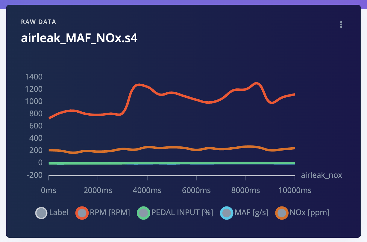
Leak hypothesis: With unmetered air, mixture trends lean > NOx is higher than expected for the same load.
2 Capture Options

Safety note: Induce a small, reversible leak (loosen an intake boot or remove a tiny vacuum cap). unplug the airflow sensor (MAF/MAP) : this can trigger limp mode and confound data.
3 Data capture (reproducible method)
Capture- Sampling: 2 Hz (every 500 ms).
- Drive cycle: idle > gentle accelerations > light cruise > decel.
- Classes:
healthy: intact intake, warmed-up closed loop.airleak_nox: the same drive cycle with a small, controlled leak.
- Windows: 2000 ms window, 1000 ms step (overlapping).
- Duration target: ~10 min per class (balanced).
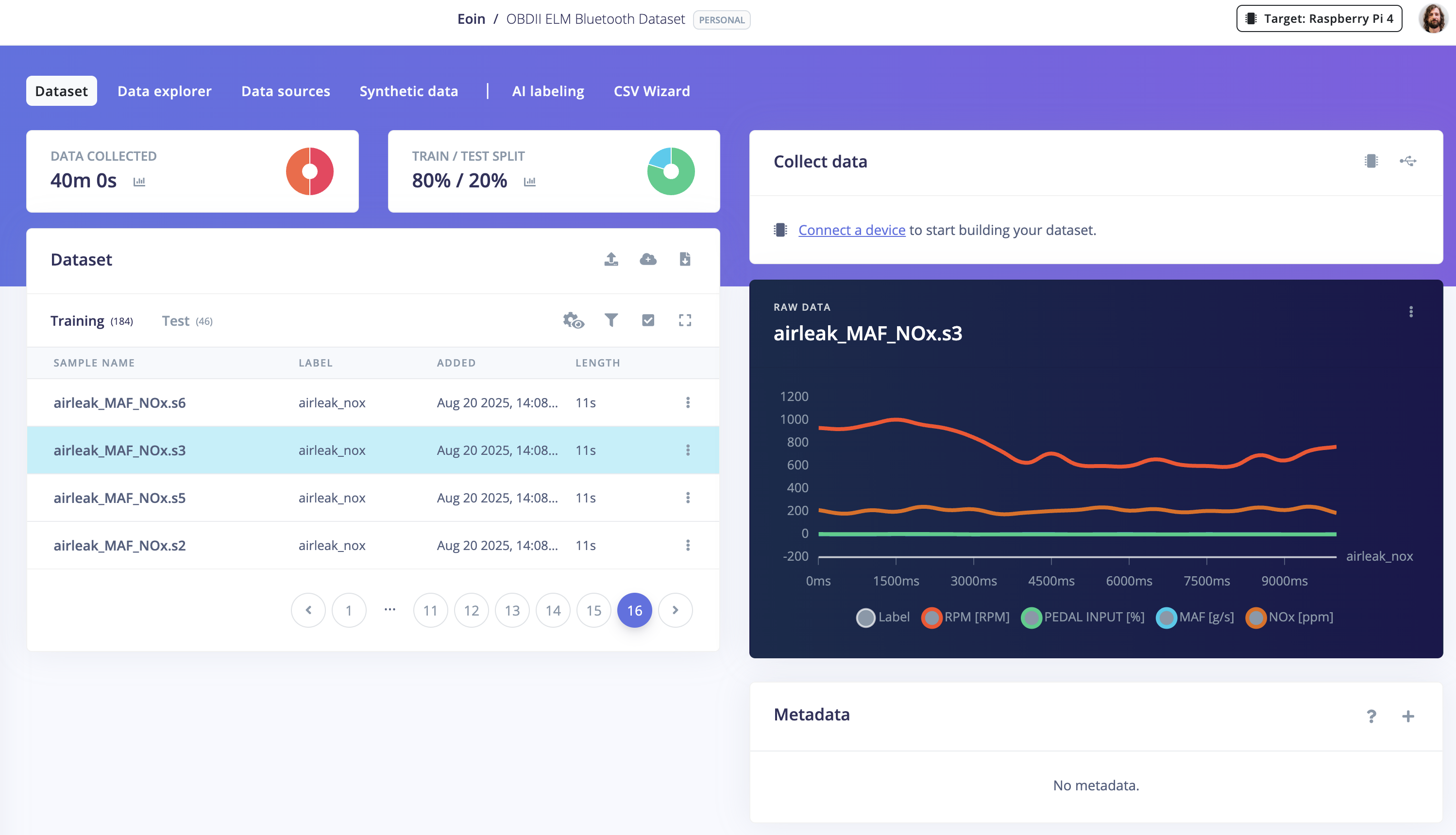
4
Healthy window example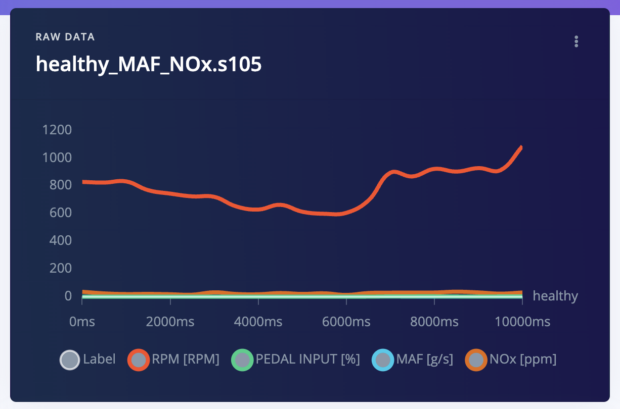
5 Simple, interpretable features (used by the classifier)
Over each 2 s window, compute:nox_per_maf = NOx / max(MAF, 0.1)nox_per_throttle = NOx / max(throttle, 1)maf_per_rpm = MAF / max(RPM, 500)- Short-window mean and **slope ** for NOx and MAF
nox_per_maf and/or positive NOx slope at modest load are more likely air-leak.
With the signals defined, wiring settled, and an explicit labeling protocol, we can now build the model.
2. Prepare the CSV
The CSV Wizard expects:- A time column named
time (ms.)(milliseconds since the first sample) - One label column (here
fault_label) - One numeric column per OBD signal
Take the sample CSV to get started or collect a sample from your OBD-II interface using your pi and the telemetry-obd project.The CSVs for the sample project have the following headings:
3. Import with the CSV Wizard
1.Open your project Data acquisition CSV Wizard2. Upload
n53_healthy_ei.csv and n53_faulty_ei.csv (or your own files)3. Set Label column =
fault_label and Time column = time (ms.)4. Confirm sampling rate ≈ 2 Hz (every 500 ms)
5. Finish import : the wizard converts each file into time-aligned samples
4. Windowing (time-series slicing)
Use windows long enough for trims/lambda to show trends:- Window size:
3000 ms - Window increase:
1500 ms
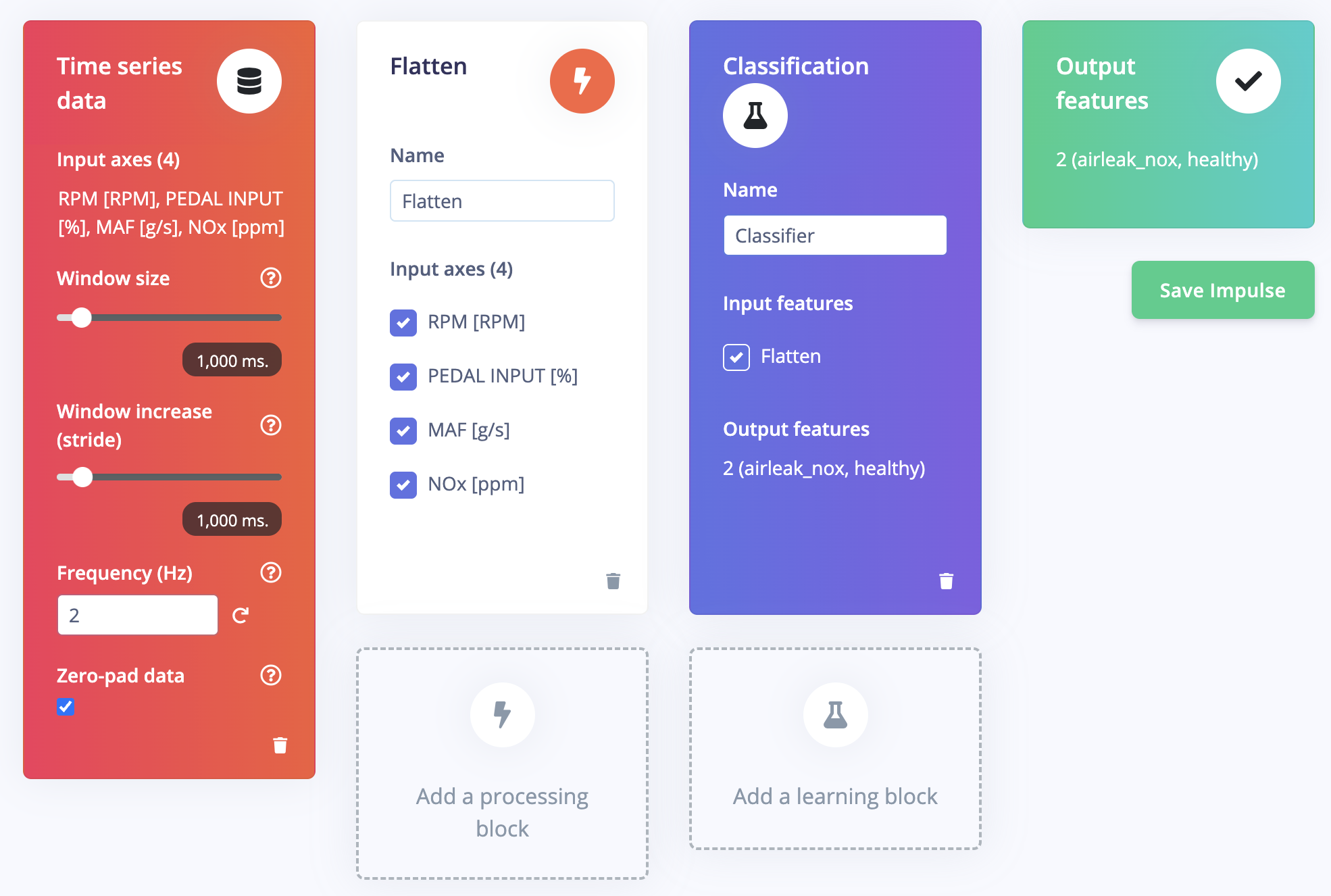
5. Create the impulse
- Go to Create impulse
- Input: your time-series window
- Processing block: Flatten (start simple)
- (Optional) add Spectral features for fast-changing channels (e.g.,
mass_air_flow_gps,nox_sensor_ppm) - (Optional) enable Normalization if feature scales differ by ≥10×
- (Optional) add Spectral features for fast-changing channels (e.g.,
- Learning block: Classification (Keras)
Start with Flatten only. If accuracy plateaus, add Spectral features as a second block.
6. Generate features
Open Generate features and run on all samples.Use Feature explorer to verify clusters separate (healthy vs. fault).
7. Train the classifier
In Classification (Keras):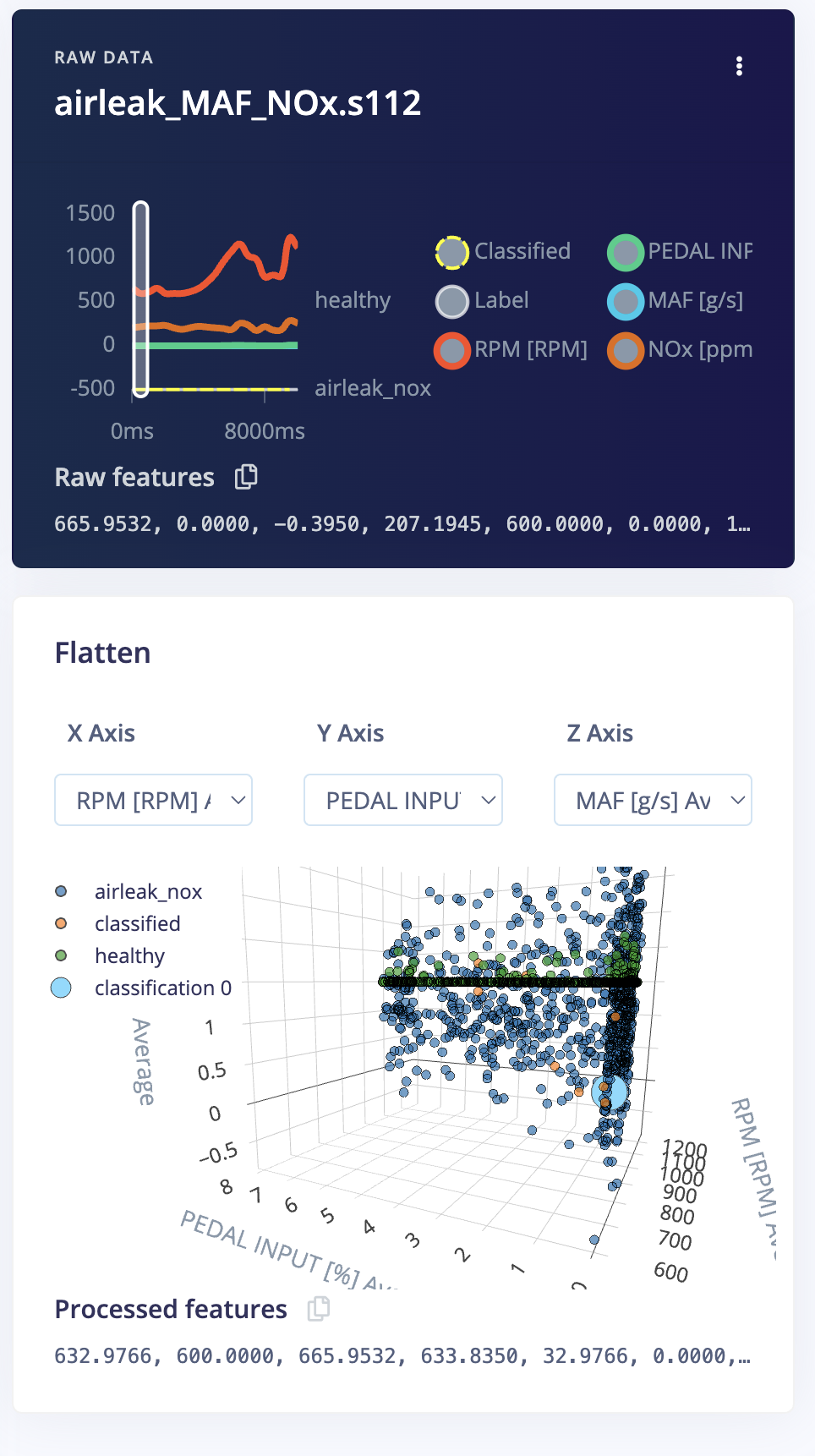
- Dense 128 (ReLU) Dropout 0.20
- Dense 64 (ReLU)
- Dense N_classes (Softmax)
- Split: 70/30 train/validation
- Epochs: 50–100
- Batch size: 32
- Enable Class weighting if classes are imbalanced
Target: ≥ 95% precision/recall per class on the validation set.
- Confusion matrix: identify misclassifications (e.g., healthy fault)
- Feature explorer: confirm separation (trims/lambda/MAF/MAP)
- If one sensor dominates (e.g., only NOx), add more context:
- STFT/LTFT (fuel trims)
- Lambda (bank1/2)
- Ratios (e.g.,
maf_per_rpm,map_per_throttle)
9. Deploy
Open Deploy and choose your target:- Linux/Aarch64 (Raspberry Pi4)